
## Introduction
Houdini by SideFX is distinctive in digital content creation. Unlike many traditional 3D applications, Houdini is based on a procedural, node-based workflow, offering artists substantial control, flexibility, and repeatability. Instead of destructive edits, users build adjustable networks that can be revised at any stage, making it especially valuable for simulation-heavy workflows.
Because of these features, Houdini is prevalent across various industries. In film and television, it is commonly used for effects like smoke, fire, fluids, and large-scale destruction. In game development, it is often used for procedural asset creation and environment generation. It’s also utilized in motion graphics, architectural visualization, and real-time pipelines where procedural workflows can significantly reduce manual effort.
At Puget Systems, Houdini isn’t new to us. We’ve monitored its progress over the years and collaborated with customers employing it in production environments. Earlier this year, we featured a guest article examining Houdini performance from a production standpoint. What is new is our capacity to rigorously and systematically test Houdini.
This post introduces the first phase of that endeavor.
## Benchmark Structure
Designing a benchmark for Houdini posed the initial challenge of determining what to measure.
Unlike many applications focused on fixed workflows, Houdini is highly procedural. Performance can vary significantly depending on the solver used, the network construction, and the simulation’s overall scale. Consequently, a single scene or task can’t fully represent real-world usage.
For this initial version, we concentrated on a select group of simulation types common in production environments, including smoke, fire, grains, fluids, and rigid body fracturing. Each simulation stresses the system differently, helping reveal performance differences across various simulation behaviors rather than a single narrow case.
All test scenes are derived from publicly available project files, with minor adjustments to improve consistency and ensure reliable benchmarking.
## Test Scenarios
Each simulation employs a specific solver with unique interactions.
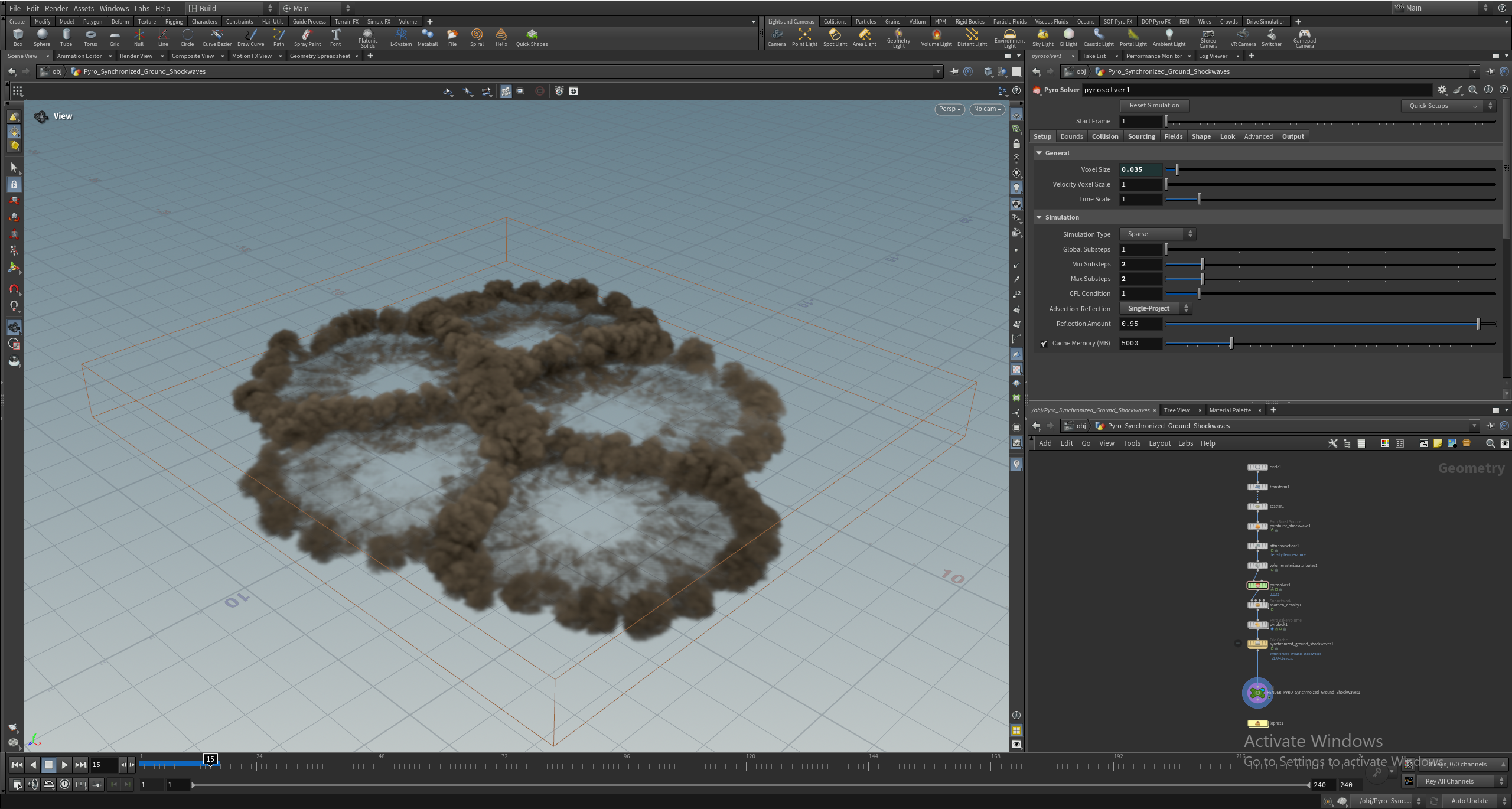
### Smoke
The Smoke simulation uses the Pyro solver, featuring five explosion points, each forming smoke clouds that interact. This replicates multiple interactive effects typical in VFX workflows, running for 240 frames from the initial explosion to the smoke’s dissipation.
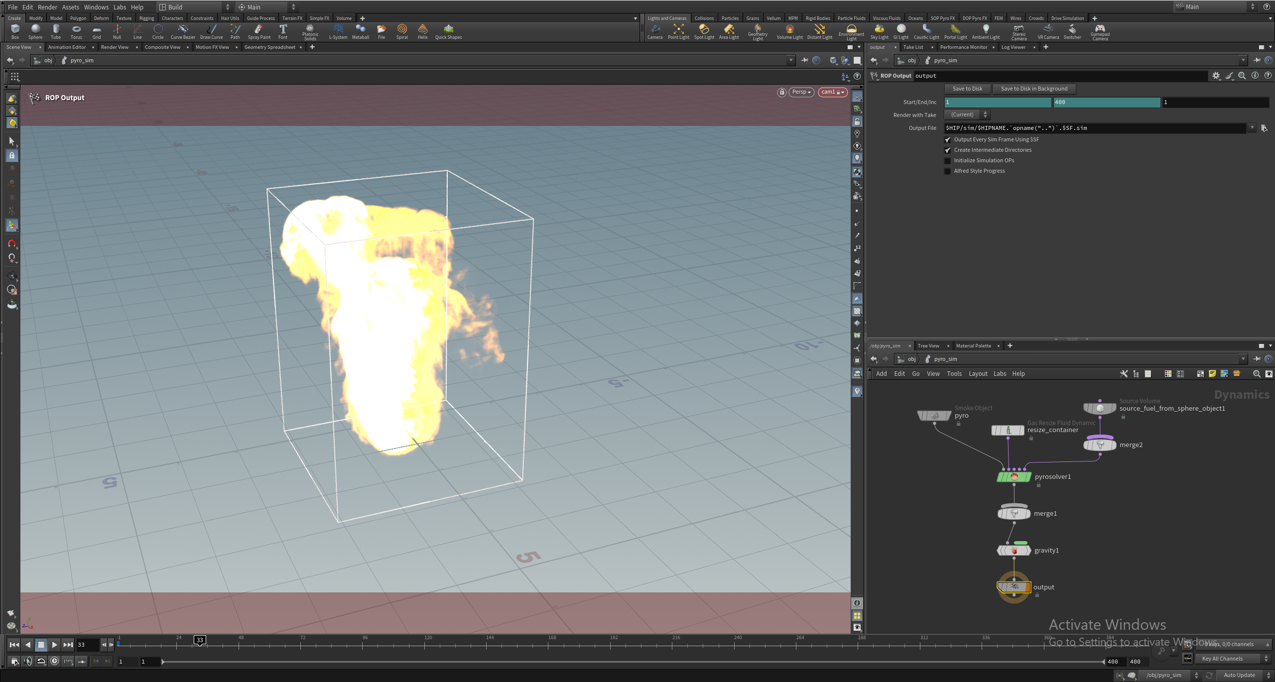
### Fire
The Fire project also uses the Pyro solver and originates from our collaborator [Saad Moosajee](https://www.pugetsystems.com/blog/2025/02/24/sidefx-houdini-performance-analysis-and-lessons-from-production/). Featuring a single flame replication, this general test runs for 200 frames.
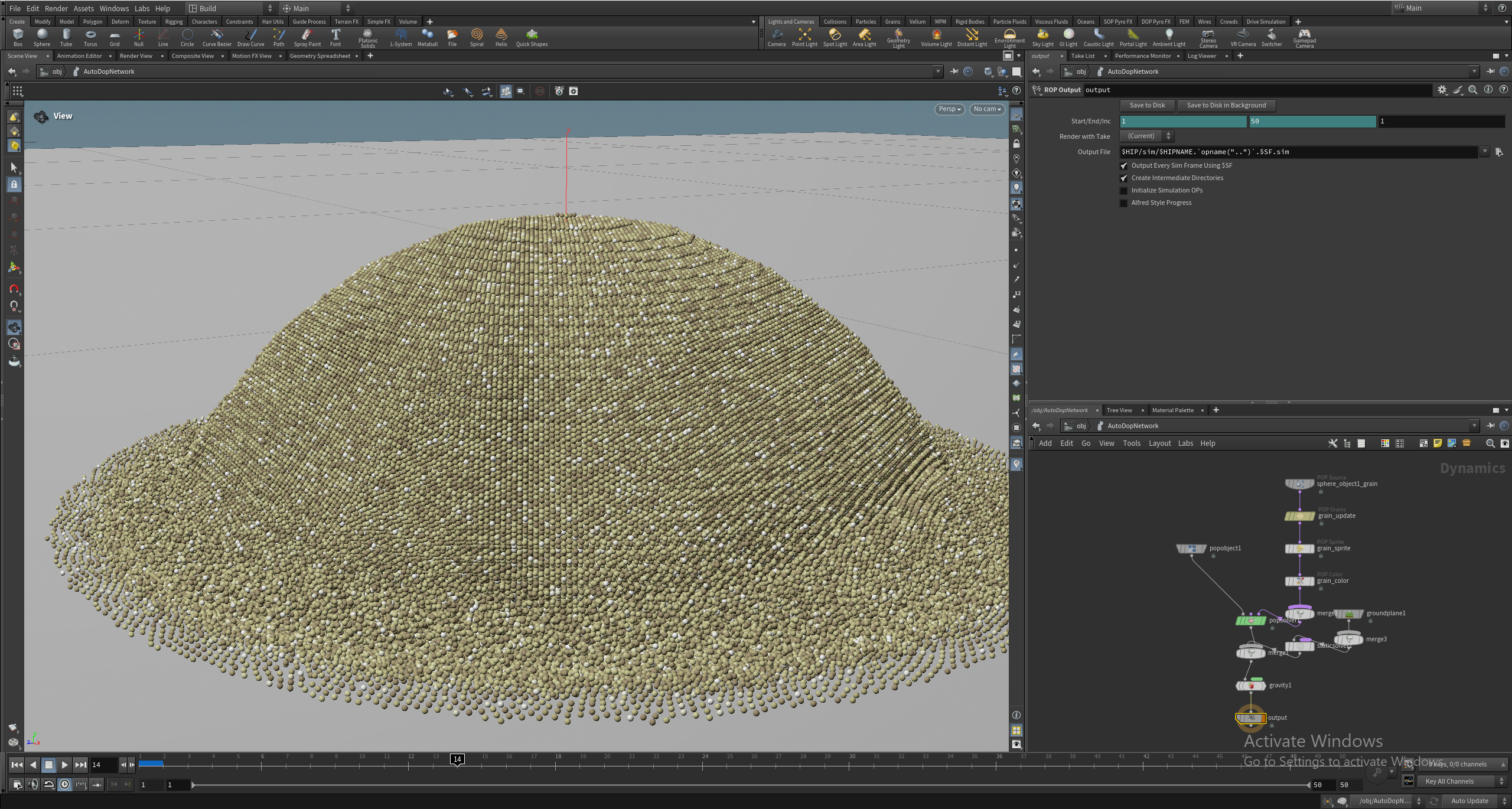
### Grains
Our Grains project, also from Saad, includes 700,000 particles created with the POP Grains node and simulated with the POP Solver node. The grains fall and scatter across a ground plane. Due to numerous interactions, this demanding test runs for 50 frames but takes nearly twice as much time as the Pyro tests.
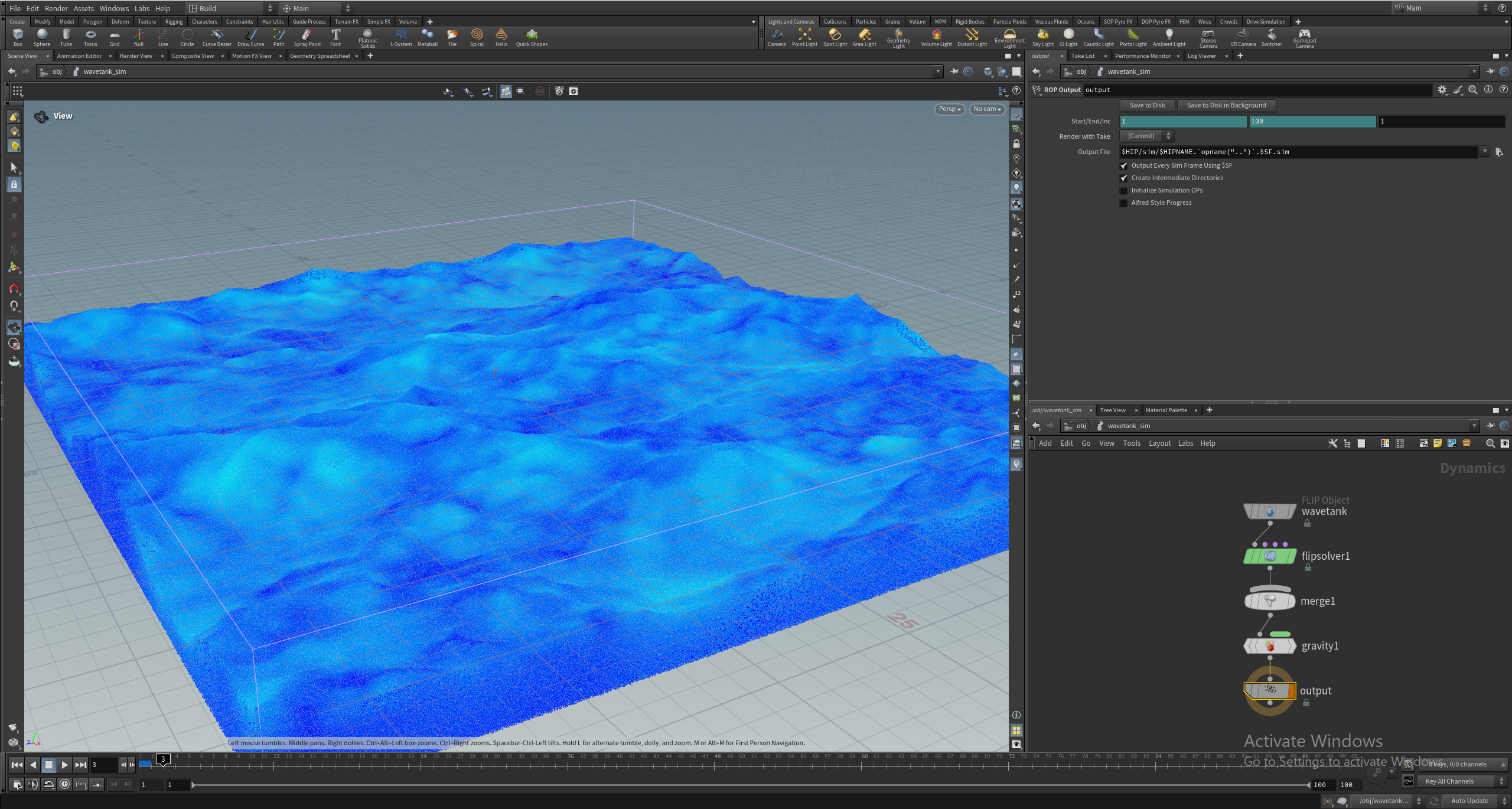
### Fluids
The Fluids test from Saad features a fluid simulation with 31 million points using the FLIP solver. Houdini excels at these simulations, frequently employed in the VFX industry for realistic water. It runs for 25 frames but takes about four times longer than the Smoke project’s 240 frames.
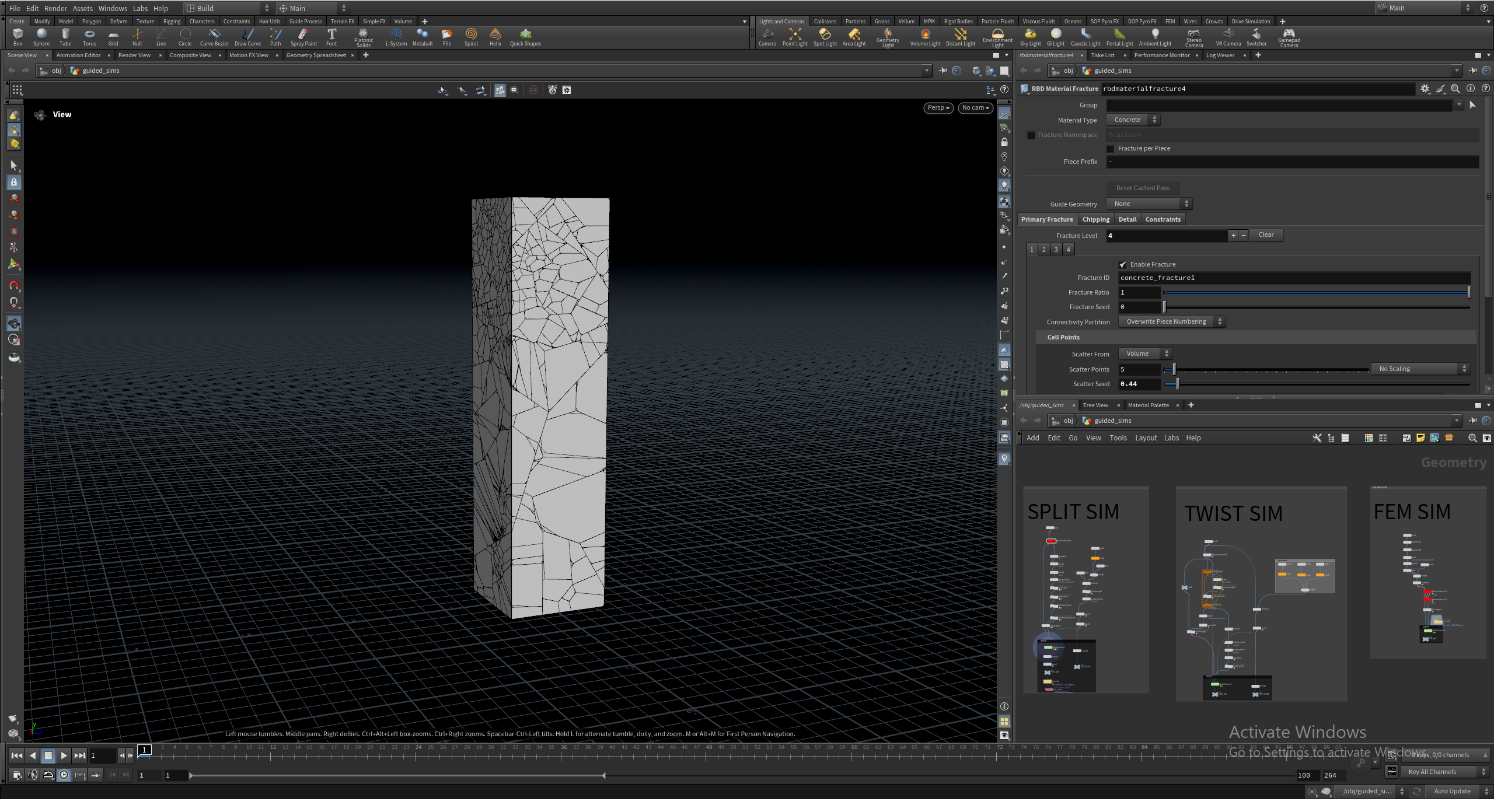
### Fracture
The Fracture test involves fracturing a large geometry with the RBD Material Fracture node and simulating its crumbling with the RBD Bullet Solver. This type is common in films and games for scenes of buildings crumbling or exploding. It runs for 100 frames.
The frame counts reflect each simulation’s characteristics. Some workloads, like Fire, require longer runtimes to capture performance behavior, while others, like Grains, quickly reach meaningful computational load, avoiding unnecessary length. This balance keeps test time reasonable while still representing each workflow’s performance profile.
## Running the Tests
All simulations run using Houdini’s *hbatch* tool in a headless environment. Running headless removes the user interface overhead, ensuring results reflect simulation performance directly. This approach mirrors many production environments where simulations run in the background or on dedicated systems.
This method provides